Toroidal coordinates

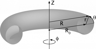
A simple toroidal coordinate system

Coordinate systems used in toroidal systems:

Cartesian coordinates

(X, Y, Z)

Cylindrical coordinates

(R, φ, Z), where

• R² = X² + Y², and
• tan φ = Y/X.

φ is called the toroidal angle (and not the cylindrical angle, at least not in the context of magnetic confinement).

Cylindrical symmetry (symmetry under rotation over φ) is referred to as axisymmetry.

Simple toroidal coordinates

(r, φ, θ), where

• R = R₀ + r cos θ, and
• Z = r sin θ

R₀ corresponds to the torus axis and is called the major radius, while r is called the minor radius, and θ the poloidal angle.

In order to adapt this simple system better to the magnetic surfaces of an axisymmetric MHD equilibrium, it may be enhanced by

• letting R₀ depend on r (to account for the Shafranov shift of flux surfaces)
• adding ellipticity (ε), triangularity (κ), etc. (to account for non-circular flux surface cross sections)

Toroidal coordinates

(ζ, η, φ), where

$R=R_{p}{\frac {\sinh \zeta }{\cosh \zeta -\cos \eta }}$

$Z=R_{p}{\frac {\sin \eta }{\cosh \zeta -\cos \eta }}$

where R_p is the pole of the coordinate system. Surfaces of constant ζ are tori with major radii R = R_p/tanh ζ and minor radii r = R_p/sinh ζ. At R = R_p, ζ = ∞, while at infinity and at R = 0, ζ = 0. The coordinate η is a poloidal angle and runs from 0 to 2π. This system is orthogonal.

The Laplace equation separates in this system of coordinates, thus allowing an expansion of the vacuum magnetic field in toroidal harmonics.

General curvilinear coordinates

Here we briefly review the basic definitions of a general curvilinear coordinate system for later convenience when discussing toroidal flux coordinates and magnetic coordinates.

Function coordinates and basis vector

Given the spatial dependence of a coordinate set $(\psi (\mathbf {x} ),\theta (\mathbf {x} ),\phi (\mathbf {x} ))$ we can calculate the contravariant basis vectors

$\mathbf {e} ^{i}=\{\nabla \psi ,\nabla \theta ,\nabla \phi \}$

and the dual covariant basis defined as

$\mathbf {e} _{i}={\frac {\partial \mathbf {x} }{\partial {u^{i}}}}\to \mathbf {e} _{i}\cdot \mathbf {e} ^{j}=\delta _{i}^{j}\to \mathbf {e} _{i}={\frac {\mathbf {e} ^{j}\times \mathbf {e} ^{k}}{|\mathbf {e} ^{i}\cdot \mathbf {e} ^{j}\times \mathbf {e} ^{k}|}}={\sqrt {g}}\;\mathbf {e} ^{j}\times \mathbf {e} ^{k}~,$

where $(i,j,k)$ are cyclic permutations of $(1,2,3)$ and we have used the notation $(u^{1},u^{2},u^{3})=(\psi ,\theta ,\phi )$. The Jacobian ${\sqrt {g}}$ is defined below.

Any vector field $\mathbf {B}$ can be represented as

$\mathbf {B} =(\mathbf {B} \cdot \mathbf {e} ^{i})\mathbf {e} _{i}=B^{i}\mathbf {e} _{i}$

or

$\mathbf {B} =(\mathbf {B} \cdot \mathbf {e} _{i})\mathbf {e} ^{i}=B_{i}\mathbf {e} ^{i}~.$

In particular any basis vector $\mathbf {e} _{i}=(\mathbf {e} _{i}\cdot \mathbf {e} _{j})\mathbf {e} ^{j}$. The metric tensor is defined as

$g_{ij}=\mathbf {e} _{i}\cdot \mathbf {e} _{j}\;;\;g^{ij}=\mathbf {e} ^{i}\cdot \mathbf {e} ^{j}\;;\;g_{i}^{j}=\mathbf {e} _{i}\cdot \mathbf {e} ^{j}=\delta _{i}^{j}~.$

Jacobian

The Jacobian of the coordinate transformation $\mathbf {x} (\psi ,\theta ,\phi )$ is defined as

$J=\det \left({\frac {\partial (x,y,z)}{\partial (\psi ,\theta ,\phi )}}\right)={\frac {\partial \mathbf {x} }{\partial {\psi }}}\cdot {\frac {\partial \mathbf {x} }{\partial {\theta }}}\times {\frac {\partial \mathbf {x} }{\partial {\phi }}}$

and that of the inverse transformation

$J^{-1}=\det \left({\frac {\partial (\psi ,\theta ,\phi )}{\partial (x,y,z)}}\right)=\nabla {\psi }\cdot \nabla {\theta }\times \nabla {\phi }$

It can be seen that $g\equiv \det(g_{ij})=J^{2}\Rightarrow J={\sqrt {g}}$

Flux coordinates

A flux coordinate set is one that includes a flux surface label as a coordinate. A flux surface label is a function that is constant and single valued on each flux surface. In our naming of the general curvilinear coordinates we have already adopted the usual flux coordinate convention for toroidal equilibrium with nested flux surfaces with $\psi$ being the flux surface label and $\theta ,\phi$ are $2\pi$-periodic poloidal and toroidal-like angles.

Different flux surface labels can be chosen like toroidal or poloidal magnetic fluxes or the volume contained within the flux surface. By single valued we mean to ensure that any flux label $\psi _{1}=f(\psi _{2})$ is a monotonous function of any other flux label $\psi _{2}$, so that the function $f$ is invertible at least in a volume containing the region of interest.

Flux Surface Average

The flux surface average of a function $\Phi$ is defined as the limit

$\langle \Phi \rangle =\lim _{\delta V\to 0}{\frac {1}{\delta V}}\int _{\delta V}\Phi \;dV$

where $\delta V$ is the volume confined between two flux surfaces. It is therefore a volume average over an infinitesimal spatial region rather than a surface average.

Introducing the differential volume element $dV={\sqrt {g}}d\psi d\theta d\phi$

$\langle \Phi \rangle =\lim _{\delta V\to 0}{\frac {1}{\delta V}}\int _{\delta V}\Phi \;{\sqrt {g}}d\psi d\theta d\phi ={\frac {d\psi }{dV}}\int _{0}^{2\pi }\int _{0}^{2\pi }\Phi \;{\sqrt {g}}d\theta d\phi$

or, noting that $\langle 1\rangle =1$, we have ${\frac {dV}{d\psi }}=\int _{0}^{2\pi }\int _{0}^{2\pi }{\sqrt {g}}d\theta d\phi$ and we get to a more practical form of the Flux Surface Average

$\langle \Phi \rangle ={\frac {\int _{0}^{2\pi }\int _{0}^{2\pi }\Phi \;{\sqrt {g}}d\theta d\phi }{\int _{0}^{2\pi }\int _{0}^{2\pi }{\sqrt {g}}d\theta d\phi }}$

Note that $dS=|\nabla \psi |{\sqrt {g}}d\theta d\phi$, so the FSA is a surface integral weighted by $|\nabla V|^{-1}$ :

$\langle \Phi \rangle ={\frac {d\psi }{dV}}\int _{0}^{2\pi }\int _{0}^{2\pi }\Phi \;{\sqrt {g}}d\theta d\phi ={\frac {d\psi }{dV}}\int _{S(\psi )}{\frac {\Phi }{|\nabla \psi |}}\;dS=\int _{S(\psi )}{\frac {\Phi }{|\nabla V|}}\;dS$

Applying Gauss' theorem to the definition of FSA we get to the identity

$\langle \nabla \cdot \Gamma \rangle =\lim _{\delta V\to 0}{\frac {1}{\delta V}}\int _{\delta V}\nabla \cdot \Gamma \;dV=\lim _{\delta V\to 0}{\frac {1}{\delta V}}\int _{S(\delta V)}\Gamma \cdot {\frac {\nabla V}{|\nabla V|}}dS=\lim _{\delta V\to 0}{\frac {1}{\delta V}}\int _{0}^{2\pi }\int _{0}^{2\pi }\Gamma \cdot \nabla V\;{\sqrt {g}}d\theta d\phi ={\frac {d}{dV}}\langle \Gamma \cdot \nabla V\rangle ~.$

Useful properties of FSA

Some useful properties of the FSA are

• $\langle \nabla \cdot \Gamma \rangle ={\frac {d}{dV}}\langle \Gamma \cdot \nabla V\rangle ={\frac {1}{V'}}{\frac {d}{d\psi }}V'\langle \Gamma \cdot \nabla \psi \rangle$
• $\int _{V}\nabla \cdot \Gamma \;dV=\langle \Gamma \cdot \nabla V\rangle =V'\langle \Gamma \cdot \nabla \psi \rangle$
• $\langle {\sqrt {g}}^{-1}\rangle ={\frac {4\pi ^{2}}{V'}}$
• $\langle \mathbf {B} \cdot \nabla f\rangle =0~,\qquad \forall ~\mathrm {single~valued~} f(\mathbf {x} ),~\mathrm {if} ~\nabla \cdot \mathbf {B} =0~\mathrm {and} ~\nabla V\cdot \mathbf {B} =0$
• $\langle \mathbf {B} \cdot \nabla \theta \rangle =2\pi {\frac {d\Psi _{pol}}{dV}}\qquad (\mathrm {Note:} ~\theta (\mathbf {x} )~\mathrm {is~not~single~valued} )$
• $\langle \mathbf {B} \cdot \nabla \phi \rangle =2\pi {\frac {d\Psi _{tor}}{dV}}\qquad (\mathrm {Note:} ~\phi (\mathbf {x} )~\mathrm {is~not~single~valued} )$

where $V'={\frac {dV}{d\psi }}$.

Magnetic field representation in flux coordinates

Contravariant From

Any solenoidal vector field $\mathbf {B}$ can be written as $\mathbf {B} =\nabla \alpha \times \nabla \nu$ called its Clebsch representation. For a magnetic field with flux surfaces $(\psi =\mathrm {const} \;,\;\nabla \psi \cdot \mathbf {B} =0)$ we can choose, say, $\alpha$ to be the flux surface label $\psi$

$\mathbf {B} =\nabla \psi \times \nabla \nu$

Field lines are then given as the intersection of the constant-$\psi$ and constant-$\nu$ surfaces. This form provides a general expression for $\mathbf {B}$ in terms of the covariant basis vectors of a flux coordinate system

$\mathbf {B} ={\frac {\partial \nu }{\partial \theta }}\nabla \psi \times \nabla \theta +{\frac {\partial \nu }{\partial \phi }}\nabla \psi \times \nabla \phi ={\frac {1}{\sqrt {g}}}{\frac {\partial \nu }{\partial \theta }}\mathbf {e} _{\phi }-{\frac {1}{\sqrt {g}}}{\frac {\partial \nu }{\partial \phi }}\mathbf {e} _{\theta }=B^{\phi }\mathbf {e} _{\phi }+B^{\theta }\mathbf {e} _{\theta }~.$

in terms of the function $\nu$, sometimes referred to as the magnetic field's stream function.

It is worthwhile to note that the Clebsch form of $\mathbf {B}$ corresponds to a magnetic vector potential $\mathbf {A} =\nu \nabla \psi$ (or $\mathbf {A} =\psi \nabla \nu$ as they differ only by the Gauge transformation $\mathbf {A} \to \mathbf {A} -\nabla (\psi \nu )$).

The general form of the stream function is

$\nu (\psi ,\theta ,\phi )={\frac {1}{2\pi }}({\dot {\Psi }}_{tor}\theta -{\dot {\Psi }}_{pol}\phi )+{\tilde {\nu }}(\psi ,\theta ,\phi )$

where ${\tilde {\nu }}$ is a differentiable function periodic in the two angles. This general form can be derived by using the fact that $\mathbf {B}$ is a physical function (hence singe-valued). The specific form for the coefficients in front of the secular terms (i.e. the non-periodic terms) can be obtained from the FSA properties .

Covariant Form

If we consider an equilibrium magnetic field such that $\mathbf {j} \times \mathbf {B} \propto \nabla \psi$, then both $\mathbf {B} \cdot \nabla \psi =0$ and $\nabla \times \mathbf {B} \cdot \nabla \psi =0$ and the magnetic field can be written as

$\mathbf {B} =\beta \nabla \psi +\nabla \chi$

where $\chi$ is identified as the magnetic scalar potential. Its general form is

$\chi (\psi ,\theta ,\phi )={\frac {I_{tor}}{2\pi }}\theta +{\frac {I_{pol}^{d}}{2\pi }}\phi +{\tilde {\chi }}(\psi ,\theta ,\phi )$

In fact, noting that

$\int _{S}\mu _{0}\mathbf {j} \cdot d\mathbf {S} =\int _{\partial S}\mathbf {B} \cdot d\mathbf {l} =\oint (\beta \nabla \psi +\nabla \chi )\cdot d\mathbf {l} =\oint (\beta d\psi +d\chi )$

and choosing an integration circuit contained within a flux surface we get

$\int _{S}\mu _{0}\mathbf {j} \cdot d\mathbf {S} =\Delta \chi ={\frac {I_{tor}}{2\pi }}\Delta \theta +{\frac {I_{pol}^{d}}{2\pi }}\Delta \phi ~.$

Sample integration circuits for the current definitions.

If we now chose a toroidal circuit $(\Delta \theta =0,\Delta \phi =2\pi )$ we get

$I_{pol}^{d}=\int _{S}\mu _{0}\mathbf {j} \cdot d\mathbf {S} \;;~\mathrm {with} ~\partial S~\mathrm {such~that} ~(\Delta \theta =0,\Delta \phi =2\pi )~.$

here the superscript $d$ is meant to indicate the flux is computed through a disc limited by the integration line, as opposed to the ribbon limited by the integration line on one side and the magnetic axis on the other that was used for the definition of poloidal magnetic flux $\Psi _{po}l$ above these lines. Similarly

$I_{tor}=\int _{S}\mu _{0}\mathbf {j} \cdot d\mathbf {S} \;;~\mathrm {with} ~\partial S~\mathrm {such~that} ~(\Delta \theta =2\pi ,\Delta \phi =0)~.$

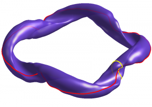
Magnetic coordinates

Magnetic coordinates adapt to the magnetic field, and therefore to the MHD equilibrium (also see Flux surface). Magnetic coordinates simplify the description of the magnetic field. In 3 dimensions (not assuming axisymmetry), the most commonly used coordinate systems are:

• Hamada coordinates. In these coordinates, both the field lines and current lines corresponding to the MHD equilibrium are straight.
• Boozer coordinates. In these coordinates, the field lines corresponding to the MHD equilibrium are straight.

These two coordinate systems are related.

References

- ↑ Wikipedia:Cartesian coordinate system
- ↑ Wikipedia:Cylindrical coordinate system
- ↑ R.L. Miller et al, Noncircular, finite aspect ratio, local equilibrium model, Phys. Plasmas 5 (1998) 973
- ↑ R.D. Hazeltine, J.D. Meiss, Plasma confinement, Courier Dover Publications (2003) ISBN 0486432424
- ↑ Morse and Feshbach, Methods of theoretical physics, McGraw-Hill, New York, 1953 ISBN 007043316X
- ↑ Wikipedia:Toroidal coordinates
- ↑ F. Alladio, F. Chrisanti, Analysis of MHD equilibria by toroidal multipolar expansions, Nucl. Fusion 26 (1986) 1143
- ↑ B.Ph. van Milligen and A. Lopez Fraguas, Expansion of vacuum magnetic fields in toroidal harmonics, Computer Physics Communications 81, Issues 1-2 (1994) 74-90
- ↑ 9.0 9.1 W.D. D'haeseleer, Flux coordinates and magnetic field structure: a guide to a fundamental tool of plasma theory, Springer series in computational physics, Springer-Verlag (1991) ISBN 3540524193
- ↑ S. Hamada, Nucl. Fusion 2 (1962) 23
- ↑ J.M. Greene and J.L Johnson, Stability Criterion for Arbitrary Hydromagnetic Equilibria, Phys. Fluids 5 (1962) 510
- ↑ A.H. Boozer, Plasma equilibrium with rational magnetic surfaces, Phys. Fluids 24 (1981) 1999
- ↑ A.H. Boozer, Establishment of magnetic coordinates for a given magnetic field, Phys. Fluids 25 (1982) 520
- ↑ K. Miyamoto, Controlled fusion and plasma physics, Vol. 21 of Series in
Plasma Physics, CRC Press (2007) ISBN 1584887095