General curvilinear coordinates
Here we briefly review the basic definitions of a general curvilinear coordinate system for later convenience when discussing toroidal flux coordinates and magnetic coordinates.
Function coordinates and basis vector
Given the spatial dependence of a coordinate set  we can calculate the contravariant basis vectors

and the dual covariant basis defined as

where  are cyclic permutations of
  and we have used the notation
  . The Jacobian
  is defined below.
Any vector field  can be represented as

or

In particular any basis vector  . The metric tensor is defined as

Jacobian
The Jacobian of the coordinate transformation  is defined as

and that of the inverse transformation

It can be seen that [1] 
Flux coordinates
A flux coordinate set is one that includes a flux surface label as a coordinate. A flux surface label is a function that is constant and single valued on each flux surface. In our naming of the general curvilinear coordinates we have already adopted the usual flux coordinate convention for toroidal equilibrium with nested flux surfaces with  being the flux surface label and
  are
are  -periodic poloidal and toroidal-like angles.
Different flux surface labels can be chosen like toroidal  or poloidal
  magnetic fluxes or the volume contained within the flux surface
  . By single valued we mean to ensure that any flux label
  is a monotonous function of any other flux label
  , so that the function
  is invertible at least in a volume containing the region of interest. We will denote a generic flux surface label by .
Flux Surface Average
The flux surface average of a function  is defined as the limit

where  is the volume confined between two flux surfaces. It is therefore a volume average over an infinitesimal spatial region rather than a surface average. To avoid confusion, we denote volume elements or domains with the calligraphic
  . Capital is reserved for the flux label (coordinate) defined as the volume within a flux surface.
Introducing the differential volume element 

or, noting that  , we have
  and
we get to a more practical form of the Flux Surface Average
and
we get to a more practical form of the Flux Surface Average

Note that  , so the FSA is a surface integral weighted by
  :
:

Applying Gauss' theorem to the definition of FSA we get to the identity

Useful properties of FSA
Some useful properties of the FSA are


where  .
.
Magnetic field representation in flux coordinates
Contravariant From
Any solenoidal vector field can be written as
 called its Clebsch representation. For a magnetic field with flux surfaces
  we can choose, say,
  to be the flux surface label

Field lines are then given as the intersection of the constant- and constant- surfaces. This form provides a general expression for in terms of the covariant basis vectors of a flux coordinate system

in terms of the function , sometimes referred to as the magnetic field's stream function.
It is worthwhile to note that the Clebsch form of corresponds to a magnetic vector potential
 (or
(or  as they differ only by the Gauge transformation
  ).
).
The general form of the stream function is

where  is a differentiable function periodic in the two angles. This general form can be derived by using the fact that is a physical function (hence singe-valued). The specific form for the coefficients in front of the secular terms (i.e. the non-periodic terms) can be obtained from the FSA properties .
Covariant Form
If we consider an equilibrium magnetic field such that  , where
  is the current density , then both
  and
and  and the magnetic field can be written as

where  is identified as the magnetic scalar potential. Its general form is

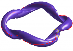
Sample integration circuits for the current definitions.
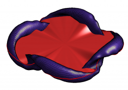
Sample surface for the definition of the current though a disc. Note that only the current of more external surfaces contribute to the flux of charge through the surface.
The functional dependence on the angular variables is again motivated by the single-valuedness of the magnetic field. The particular form of the coefficients can be obtained noting that

and choosing an integration circuit contained within a flux surface  . Then we get

If we now chose a toroidal circuit  we get

here the superscript  is meant to indicate the flux is computed through a disc limited by the integration line, as opposed to the ribbon limited by the integration line on one side and the magnetic axis on the other that was used for the definition of poloidal magnetic flux
  above these lines.
Similarly
above these lines.
Similarly

Contravariant Form of the current density
Taking the curl of the covariant form of the equilibrium current density can be written as

By very similar arguments as those used for (note that both and are solenoidal fields tangent to the flux surfaces) it can be shown that the general expression for  is
is

Note that the poloidal current is now defined through a ribbon and not a disc.
Magnetic coordinates
Magnetic coordinates are a particular type of flux coordinates in which the magnetic field lines are straight lines. In mathematical terms this implies that the periodic part of the magnetic field's stream function is zero in these coordinates so the magnetic field reads

Note that, in general, the contravariant components of the magnetic field in a magnetic coordinate system

are not flux functions, but their quotient is

 being the rotational transform.
Any transformation of the angles of the from

where  is periodic in the angles, preserves the straightness of the field lines. The spatial function
  , is called the generating function.
Magnetic coordinates adapt to the magnetic field, and therefore to the MHD equilibrium (also see Flux surface).
Magnetic coordinates simplify the description of the magnetic field.
In 3 dimensions (not assuming axisymmetry), the most commonly used coordinate systems are:
[1]
- Hamada coordinates. [2][3] In these coordinates, both the field lines and current lines corresponding to the MHD equilibrium are straight. Referring to the definitions above, both and
 are zero in Hamada coordinates.
- Boozer coordinates. [4][5] In these coordinates, the field lines corresponding to the MHD equilibrium are straight and so are the diamagnetic lines , i.e. the integral lines of
 . Referring to the definitions above, both and
  are zero in Boozer coordinates.
These two coordinate systems are related.
[6]
References
- ↑ 1.0 1.1 W.D. D'haeseleer, Flux coordinates and magnetic field structure: a guide to a fundamental tool of plasma theory, Springer series in computational physics, Springer-Verlag (1991) ISBN 3540524193
- ↑ S. Hamada, Nucl. Fusion 2 (1962) 23
- ↑ J.M. Greene and J.L Johnson, Stability Criterion for Arbitrary Hydromagnetic Equilibria, Phys. Fluids 5 (1962) 510
- ↑ A.H. Boozer, Plasma equilibrium with rational magnetic surfaces, Phys. Fluids 24 (1981) 1999
- ↑ A.H. Boozer, Establishment of magnetic coordinates for a given magnetic field, Phys. Fluids 25 (1982) 520
- ↑ K. Miyamoto, Controlled fusion and plasma physics, Vol. 21 of Series in
Plasma Physics, CRC Press (2007) ISBN 1584887095

